How does DBSCAN clustering algorithm work?

the biggest secrets behind a clustering algorithm

6 min readJul 26, 2019

“If you can’t explain it simply, you don’t understand it well enough.” — **Albert Einstein**

Scikit Learn — Demo of DBSCAN clustering algorithm

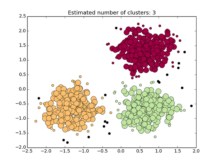
Cluster Analysis is an important problem in data analysis. And nowadays DBSCAN is one of the most popular Cluster Analysis techniques. Density-based spatial clustering of applications with noise (DBSCAN) is the data clustering algorithm proposed in the early 90s by a group of database and data mining community.

Now before we begin, let’s understand the core philosophy of DBSCAN.

Let a given dataset of points (dataset D = {xi}), we have to partition the point into the dense region which we will call them as Clusters and sparse region which may contain noise.

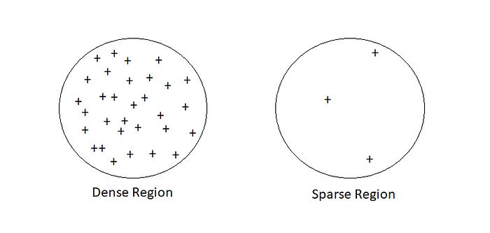
Before we can discuss density-based clustering, we first need to cover a few topics.

Parameters:

DBSCAN algorithm basically requires 2 parameters:

eps: specifies how close points should be to each other to be considered a part of a cluster. It means that if the distance between two points is lower or equal to this value (eps), these points are considered to be neighbors.

minPoints: the minimum number of points to form a dense region. For example, if we set the minPoints parameter as 5, then we need at least 5 points to form a dense region. It’s basically known as min_samples.

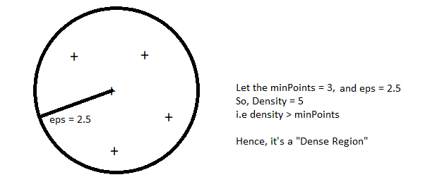
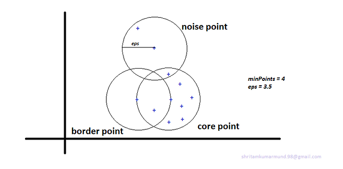
In this algorithm, we have 3 types of data points. Every point in our dataset D = {xi}, on given minPoints and eps we can categorize every data point into Core point, Border point and Noise point.

Let me define each of them.

Core point:

A point is a core point if it has more than a specified number of minPoints within eps radius around it.
Core Point always belongs in a dense region.
For example, let’s consider ‘p’ is set to be a core point if ‘p’ has ≥ minPoints in an eps radius around it.

Border point:

A point is a border point if it has fewer than MinPts within Eps, but is in the neighborhood of a core point.
For example, p is set to be a border point if ‘p’ is not a core point. i.e ‘p’ has < minPoints in eps radius. But ‘p’ should belong to the neighborhood ‘q’. Where ‘q’ is a core point.
p ∈ neighborhood of q and distance(p,q) ≤ eps .

Noise point:

A noise point is any point that is not a core point or a border point.

There are two more important ideas that we should be aware of before we go and learn the DBSCAN algorithm.

Density Edge:

If p and q both are core points and distance between (p,q) ≤ eps then we can connect p, q vertex in a graph and call it “Density Edge”.

Density Connected Points:

Two points p and q are said to be density connected points if both p and q are core points and they exist a path formed by density edges connecting point (p) to point(q).

DBSCAN algorithm:

So, given all these terms and ideas, let's go into the core of the DBSCAN algorithm to see how it works.

Algorithm:

step 1: ∀ xi ∈ D, Label points as the core, border, and noise points.

step 2: Remove or Eliminate all noise points. (because they belong to the sparse region. i.e they are not belonging to any clusters.)

step 3: For every core point p that has not yet been assigned to a cluster

a) Create a new cluster with the point p and

b) add all the points that are density-connected to p.

step 4: Assign each border points to the cluster of the closest core point.

After knowing each DBSCAN concept, The question now arises:

How to choose Min Points?

Well, one of the most important things that min Point does is to remove the outlier right!
Typically, the rule of thumb for taking min Points is, you should always take your min points to be greater or equal to the dimensionality(d) of your dataset.
Typically, people who work most with DBSCAN take min point twice of the dimensionality of data i.e min Point≈2*d.
If the dataset is noisier, we should choose a larger value of min Points
While choosing the min points, it really depends a lot on domain knowledge.

How to determine eps?

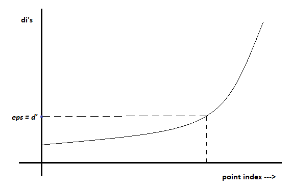
Once you choose your min Point, you can proceed with the eps.
Let us choose a min point = 4, for each point p I’ll compute “di”. where di= distance from p to the 4th nearest neighbor of p. If “di” is high, then the chance of p is noisy is also high.

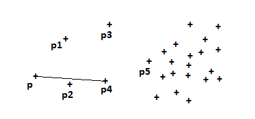
For each point in the data set, I’ll have my di’s. Now sort all di’s in increasing order.
Since we have sorted our point in the increasing order of di’s, now we’ll plot sorted point index and di’s with elbow or Knee method.

When DBSCAN work well?

It can handle Noise very well.
DBSCAN can handle clusters of different shapes and sizes.

When not!

DBSCAN, while it’s so powerful and good for some applications. There is no single algorithm that always works. Every pro has some con side.
If your dataset has multiple densities or varying densities, DBSCAN tends to fail. It does not work very well in such cases.
It’s extremely sensitive to the hyperparameters. A slight change in hyperparameters can lead to a drastic change in the outcome.
As we know, a concept like Density, may not work well in high dimensionality of data. We should avoid using it for text data.

Time and Space complexity:

Time Complexity: O(n log n)

Space Complexity: O(n)

Implementation:

We don’t need to worry about implementing it ourselves. We can use one of the libraries/packages that can be found on the internet. Also, Sklearn has a DBSCAN implemented package. Let’s see how to code.

Simple Overview:

from sklearn.cluster import DBSCAN
from sklearn import metrics
import numpy as npX = #load the data
clustering = DBSCAN(eps=3, min_samples=2).fit(X)#Storing the labels formed by the DBSCAN
labels = clustering.labels_# measure the performance of dbscan algo
#Identifying which points make up our “core points”
core_samples = np.zeros_like(labels, dtype=bool)
core_samples[clustering.core_sample_indices_] = True
print(core_samples)#Calculating "the number of clusters"
n_clusters_ = len(set(labels)) - (1 if -1 in labels else 0)
print(n_clusters_)#Computing "the Silhouette Score"
print("Silhouette Coefficient: %0.3f"
      % metrics.silhouette_score(X, labels))

Silhouette Coefficient Score:
The Silhouette Coefficient is calculated using the mean intra-cluster distance (a) and the mean nearest-cluster distance (b) for each sample. The Silhouette Coefficient for a sample is (b - a) / max(a, b). To clarify, b is the distance between a sample and the nearest cluster that the sample is not a part of. Note that Silhouette Coefficient is only defined if number of labels is 2 <= n_labels <= n_samples - 1.
This function returns the mean Silhouette Coefficient over all samples.
A silhouette score ranges from -1 to 1, with -1 being the worst score possible and 1 being the best score. Silhouette scores of 0 suggest overlapping clusters.